Micrograd

I want to walk you through the core ideas behind automatic differentiation and tiny neural networks, using the spirit of micrograd as a guide.

The goal is simple: understand how a model turns inputs into outputs, how gradients tell us what to change, and how repeated small updates can teach a network.

Why gradients?

In machine learning, a model produces an output from some inputs. If the output is not what we want, we need a way to tune it, or measure how each input or parameter affected that result. That is what a gradient does. It tells us:

• whether a small change in one variable increases or decreases the output
• how sensitive the output is to that variable
• how strongly that variable should be adjusted during training

Think of it as a direction and magnitude for improvement in terms of your output.

Estimating slope by nudging values

Let’s start with the intuition of a derivative, and for that let us consider a mathematical expression

$$L=d∗f$$

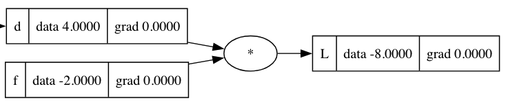
where, L = output , d and f are inputs

Before jumping into formulas, let us ask a practical question.

• If we nudge an input a tiny bit, how much does the output change?

This is the finite-difference view of slope. It is a numerical way to approximate a derivative by comparing:

• the original output
• the output after a tiny change

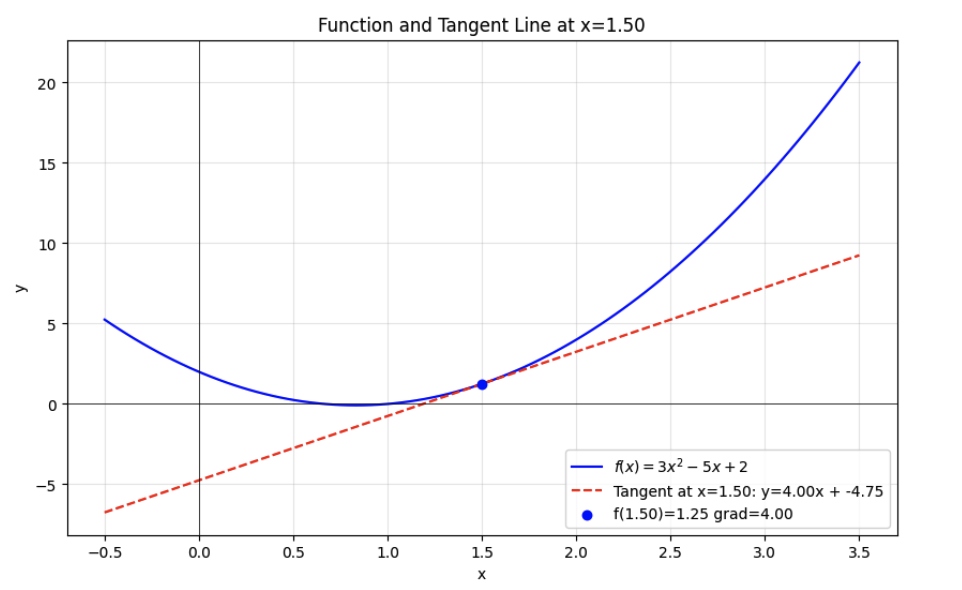
This makes gradients feel concrete before moving into calculus. The following diagram shows a slope at a particular input value of a quadratic expression.

From slope to calculus

Once this idea is clear, we can intuitively understand differentiation and work out a little math:

$$\begin{aligned} & \frac{dL}{df} = ? \\ & \lim_{h \to 0} \frac{f(x + h) - f(x)}{h} \\ & \frac{d(f + h) - (d \cdot f)}{h} \\ & \frac{df + dh - df}{h} \\ & \frac{dh}{h} = d \end{aligned}$$

The derivative of L with respect to f dL/df = d

For a simple function like a quadratic, the derivative gives the exact slope at any point. That slope changes depending on where you evaluate the function. This is important because neural networks are full of such changing relationships. We need a way to measure slope not just once, but across an entire graph of operations.

Building expressions as graphs

A key idea in micrograd is that a mathematical expression can be represented as a graph.

Each intermediate result becomes a node in the graph:

• inputs are leaf nodes
• operations create new nodes
• the final output sits at the end of the chain

This graph is useful because it shows not just the final answer, but how that answer was formed.

If we know the structure of the graph, we can move backward through it and compute gradients for every part.

Value:

Represents a small scalar object that stores:

• the numeric data
• the gradient
• the operation that produced it
• links to previous values

This tiny object is the heart of the system. It behaves like a tracked number. Whenever values are added, multiplied, exponentiated, or passed through nonlinearities, the result remembers how it was created.

That memory is what makes backpropagation possible.

class Value:
    def __init__(self, data, _children = (), _op = '', label=''):
        self.data = data
        self.grad = 0.0  # gradient or slope of the func w.r.t to this value

        self._backward = lambda: None  # function

        self._prev = _children 
        self._op = _op
        self.label = label


    def __add__(self, other):
        other = other if isinstance(other, Value) else Value(other) 
        out = Value(self.data + other.data, (self, other), _op = '+')

        def _backward():
            self.grad += 1.0 * out.grad
            other.grad += 1.0 * out.grad
        out._backward = _backward

        return out

        ...

Backpropagation in plain language

Backpropagation answers the question: How does the final output change if one earlier value changes?

Process:

• start from the output, say L
• set its gradient to 1 (intuitively, changing L affects itself by a factor of 1)
• walk backward through the graph to trace gradients(here, L = d * f)
• apply the chain rule at every operation (say, if d = a * b)

So, gradients flow from the output toward the inputs, one local step at a time.

From, a code perspective the _backward method represents the derivative or gradient calculation. The below one shows an example for tanh.

# Within Value Class:
    def tanh(self):
        x = self.data
        t = (math.exp(2*x) -1)/(math.exp(2*x) + 1)
        out = Value(t, (self, ), 'tanh')

        def _backward():
            self.grad += (1 - t**2) * out.grad
        out._backward = _backward

        return out

Chain rule

The chain rule is the engine that makes backpropagation work. If one value depends on another, and the final output depends on that value, then the total influence is the product of the local influences.

In practice:

• addition passes gradient evenly to both inputs
• multiplication scales each input by the other input’s value
• nonlinear functions like tanh or exp each have their own backward rule

The important takeaway is that complex derivatives are built from simple local rules. The following code backpropagates from the expression graph in reverse, calculating and updating gradients recursively at each node.

# Within Value Class
.. 
    def backward(self):

        topo = [] 
        visited = set()

        def build_topo(v):
            if v not in visited:
                visited.add(v)
                for child in v._prev:
                    build_topo(child)
                topo.append(v)

        build_topo(self)

        self.grad = 1.0
        for node in reversed(topo):
            node._backward()

A simple neural network neuron

Conceptually, a neuron does three things:

• multiplies each input by a weight
• adds a bias
• applies a nonlinearity

This turns raw numbers into a learned representation. The nonlinearity matters because without it, stacked layers would collapse into a simple linear model. Activation functions give the network expressive power.

Matching micrograd with PyTorch

PyTorch does the same essential job, but it does it at scale:

• tracks tensor operations automatically
• computes gradients efficiently
• runs on optimized hardware

The conceptual match is the important part. micrograd is a miniature version of the same idea:

• forward pass to compute output
• backward pass to compute gradients
• use the gradients to update parameters

Neuron to an MLP

An MLP (Multi-Layer Perceptron) is just layers of neurons stacked together:

• an input layer receives values
• hidden layers transform them
• an output layer produces the final prediction

Let us build a MLP with:

• input layer: 3
• intermediate or hidden layers: [4 , 4]
• output layer: 1

class Neuron:

    def __init__(self, nin):
        self.w = [Value(random.uniform(-1, 1)) for _ in range(nin)]
        self.b = Value(random.uniform(-1, 1))

    def __call__(self, x):
        # w*x + b
        act = sum((wi * xi for wi, xi in zip(self.w, x)), self.b)
        out = act.tanh()
        return out

    def parameters(self):
        return self.w + [self.b] 

class Layer:

    def __init__(self, nin, nout):
        self.neurons = [Neuron(nin) for _ in range(nout)]

    def __call__(self, x):
        outs = [n(x) for n in self.neurons]
        return outs[0] if len(outs) == 1 else outs

    def parameters(self):
        return [p for neuron in self.neurons for p in neuron.parameters()] 


class MLP:
    def __init__(self, nin, nouts):
        sz = [nin] + nouts 
        self.layers = [Layer(sz[i], sz[i+1]) for i in range(len(nouts))] 

    def __call__(self, x):
        for layer in self.layers:
            x = layer(x)
        return x 

    def parameters(self):
        return [p for layer in self.layers for p in layer.parameters()] 

Each layer contains learnable weights and biases. Together, they form a network that can model more complex patterns than a single neuron.

Training loop intuition

Training is presented as a repeating cycle:

# Initialize Network with the network assumed earlier.

x = [2.0, 3.0, -1.0]
mlp = MLP(3, [4, 4, 1])
mlp(x)

xs = [
    [2.0, 3.0, -1.0],
    [3.0, -1.0, 0.5],
    [0.5, 1.0, 1.0],
    [1.0, 1.0, -1.0],
]

ys = [1.0, -1.0, -1.0, 1.0] # desired targets

# Do it iteratively : Forward pass, Backward pass, Update Weights . 


def train_it(k):
    # Forward Pass
    ypred = [mlp(x) for x in xs]
    loss = sum((yout - ygt) ** 2 for ygt, yout in zip(ys, ypred))

    # Backward Pass
    for p in mlp.parameters():  # set to zero-grad before backpropagating.
        p.grad = 0.0
    loss.backward()

    # Update Weights
    for p in mlp.parameters():
        p.data += -0.01 * p.grad # Gradient Descent: -ve because we want to minimize the loss. 

    print ( "Y Pred:", [f"{y.data:.5f}" for y in ypred])
    print (f"Current Step: {k} , Loss: {loss}\n")

1. make predictions with the current parameters
2. compute a loss that measures error
3. clear old gradients
4. run backpropagation
5. update parameters in the direction that reduces loss

This is gradient descent in its simplest form.

The update step is small on purpose. Many small steps are usually better than one big jump, especially when the loss surface is complicated.

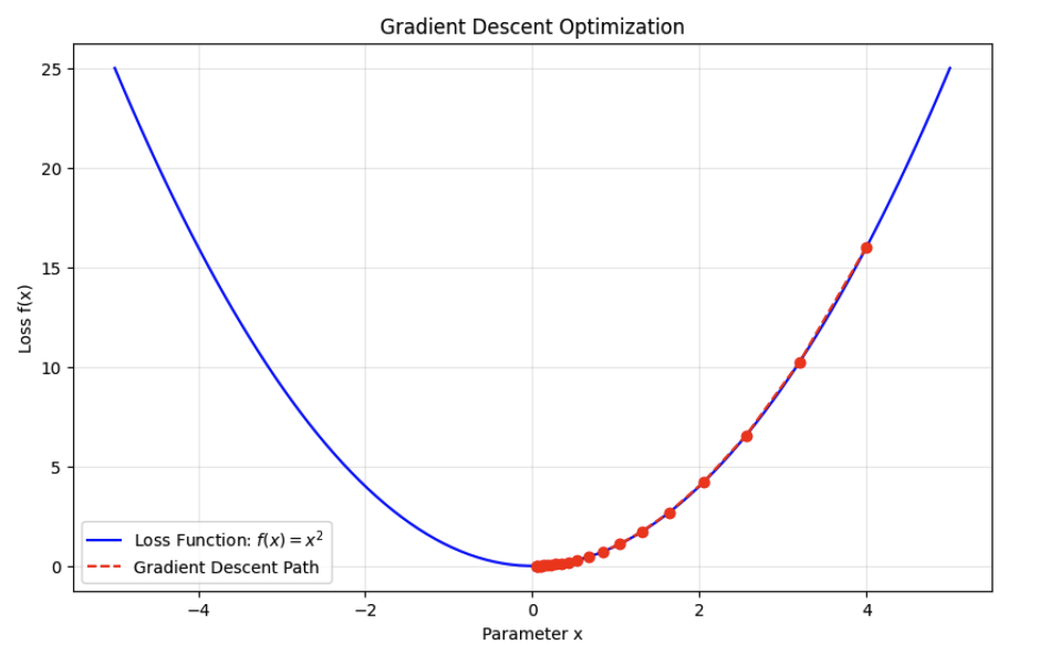
The visualization above demonstrates the optimization process seen in the train_it function.

1. Loss Function ($f(x)=x^2$): Represents the error surface we want to minimize.
2. Gradient: At any point, the slope ($2x$) tells us the direction of steepest increase.
3. Step: We move in the opposite direction of the gradient: $x_{new} = x_{old} - \text{learning\_rate} \cdot \nabla f(x)$
4. Convergence: By iteratively nudging the parameters, we descend the slope towards the global minimum (where the gradient is zero).

Further references

Notebook: micrograd/micrograd.py

The value of this marimo notebook is not just that it demonstrates a tiny neural net. It shows how modern deep learning systems are built from a few core ideas:

• numbers with memory
• graphs of computations
• the chain rule
• backward gradient flow
• iterative optimization

Once those ideas click, the behavior of larger frameworks becomes much easier to understand.

Source: https://www.youtube.com/watch?v=VMj-3S1tku0 - Andrej Karpathy

Conclusion

micrograd is a teaching tool, but it teaches a real pattern used everywhere in machine learning.

The model takes inputs, transforms them through layers of learned parameters, measures error with a loss and then uses gradients to improve itself. That loop is the foundation of neural network training. If you understand one small engine, you understand the backbone of much larger systems.